Tutorial 5: Custom Fields

This tutorial describes how to create custom quantum dark matter fields in Jaxion simulations. An example is provided in examples/two_field

First, params["physics"]["quantum"] should be set to False since we will be adding out own fields.

For example, to create a two-field simulation, we can add the simulation states: sim.state["psi1"] and sim.state["psi2"].

Then, we need to define custom kick, drift, and total density functions, and attach them to the simulation object:

def custom_density(state):
    return jnp.abs(state["psi1"]) ** 2 + jnp.abs(state["psi2"]) ** 2

def custom_kick(state, V, dt):
    state["psi1"] = jnp.exp(-1j * m1_per_hbar * dt * V) * state["psi1"]
    state["psi2"] = jnp.exp(-1j * m2_per_hbar * dt * V) * state["psi2"]

    return state

def custom_drift(state, k_sq, dt):
    psi1_hat = jd.fft.pfft3d(state["psi1"])
    psi1_hat = jnp.exp(dt * (-1.0j * k_sq / m1_per_hbar / 2.0)) * psi1_hat
    state["psi1"] = jd.fft.pifft3d(psi1_hat)

    psi2_hat = jd.fft.pfft3d(state["psi2"])
    psi2_hat = jnp.exp(dt * (-1.0j * k_sq / m2_per_hbar / 2.0)) * psi2_hat
    state["psi2"] = jd.fft.pifft3d(psi2_hat)

    return state

sim.custom_density = custom_density
sim.custom_kick = custom_kick
sim.custom_drift = custom_drift

In this example, the custom density function is used to compute the total density from both dark matter fields. The custom kick and drift functions are used to update the fields during the simulation.

The simulation can then be run as usual with sim.run().

It is also possible to add custom plotting for these fields by defining a custom plotting function and attaching it to the simulation object: custom_plot(state, checkpoint_dir, i, params).

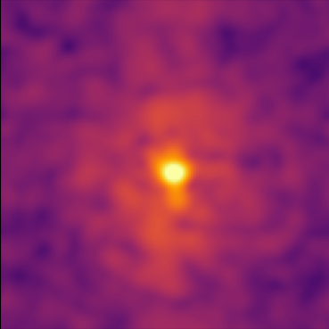
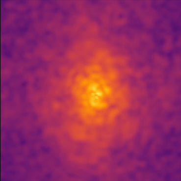
The Two-Field example evolves two quantum fields with different masses that interact gravitationally, and looks something like this: